tiredlizard's Guide to Nothing of Import

Putting the SCE in... 'Sceince': A Rushed Introduction to Single Cell Experiments

So, you woke up this morning and wondered "what in the heck is an SCE object?". Just kidding, no one does that. That's why I'm here to tell you about something you've never even heard about. My fellow students, don't be too alarmed by the '11 Minute Read'; you can skim it in, like, two minutes. (I'm very sorry.)

SCE Questions

Take a shot (of water!) every time I say ‘SCE object’.

What is the SCE object?

I’ll start with the basics. SCE stands for Single-Cell Experiment. So an SCE object, you guessed it, contains biological data for cells. “Why would you want to work with biological data?” you ask. “Because I’m a masochist,” I answer. No, I’m a biostatistican, but same difference. At least I’m not an actuary. Those guys really are masochists. (I’m joking!)

Anyways, the main assay, which is essentially a data frame of raw counts, is made up of thousands of rows representing certain genes and columns representing certain (biological) cells. The data I’m playing with here has 6,260 gene expressions (rows) and 65,246 individual cells (columns), meaning I have a grand total of a whopping 408,439,960 (table) cells. Yeah, it’s a lot. In fact, it has to use a sparse matrix - a matrix that collapses all cells with ‘0’ into commas - to save space. Even then, this particular object is about 1.3 gigabytes.

Where is the SCE object?

BiocManager is my best friend. You can’t have it.

Ugh, fine. Here’s how you’d install it:

install.packages("BiocManager", repos = "https://cloud.r-project.org")
BiocManager::install('SingleCellExperiment') # SCE objects are part of this package.

Of course, I have my actual SCE data given to me from my professor. Good luck finding some on your own!

Why is the SCE object?

(Yes, I’m ignoring proper grammar for the joke.)

The SCE object is a smaller part of something called single cell RNA sequencing (or scRNA-seq for short). In scRNA-seq, we capture the gene expression of individual cells, which helps us understand cellular differences in complex tissues or conditions like cancer. For example, my dataset is part of a larger one involving Renal Cell Carcinoma and identifying gene expressions that are more common in cells found in the cancerous regions than in cells found in the adjacent normal regions… what a mouthful. So, essentially, SCE objects serve as containers to store all this incredibly complex data.

Long story short: RNA tells us important stuff, we put the important stuff into Single-Cell Experiment objects.

How is the SCE object?

It’s doing well; thanks for asking.

Alright, I admit, this is getting old. But the structure of the Single-Cell Experiment is very important, and probably one of the most difficult things to explain.

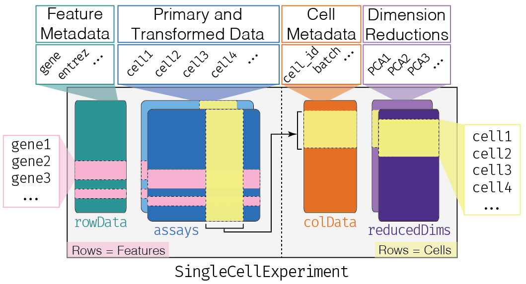
Oh, nevermind. It was pretty easy!

In all seriousness, an SCE object has an odd format. The primary assay, as mentioned before, is made of counts - it’s essentially a matrix of mostly 0s that shows which cells express which genes. But then we have… the metadata.

The metadata contains information about each cell. This is what happens when you load the column metadata on the first three cells.

load("sce.Rdata")
first.3 <- sce[,1:3]
colData(first.3)
#=> prints: 
DataFrame with 3 rows and 8 columns
                       nGene      nUMI      sample percent_mito doublet_score       batch        type       stage
                   <integer> <numeric> <character>    <numeric>     <numeric> <character> <character> <character>
AAACCTGAGAGCTTCT-9      1655      5721       S14_N 1.15962e-212    0.00133505           4           N      locAdv
AAACCTGAGTCGTTTG-9      1547      4883       S14_N  6.30512e-16    0.51172545           4           N      locAdv
AAACCTGGTGCATCTA-9      1349      2237       S14_N  5.01866e-15    0.00000000           4           N      locAdv

Where (you can skim this if you want):

• nGene: number of unique genes detected in each cell
• nUMI: number of Unique Molecular Identifiers (UMI)
• sample: indicates sample each cell belongs to
• percent_mito: percentage of UMIs that map to mitochondrial genes in each cell
• doublet_score: score estimating the likelihood that a cell is a “doublet”, meaning two cells were captured as one during sequencing
• batch: which batch the cell belongs to
• type: indicates condition of the cell (normal or tumor)
• stage: refers to stage of disease (early, locally advanced, metastatic)

Wow, I didn’t even understand most of that, and I spent six weeks with this data.

Who is the – okay, I’ll stop now.

I know, I’m hilarious. …this is probably why no one will hire me, huh. Moving on!

So now you want to analyze data.

Since I have to include some form of data science in this post, I suppose I will go over the basic things you can do with the SCE object. I am so sorry to my classmates in Stat 386. (Hopefully this counts as data science? Since it’s science… using data?)

Normalization

Unfortunately, since this is biological data, it is very much not normal. In order to perform any kind of analysis, you’re going to want to normalize it. (Sorry Python users - I’m working in R and I will not cater to your needs.)

scaled <- t(t(assay(sce, "counts")) / colSums(assay(sce,"counts"))) # Takes counts assay and divides each table cell by the sum of the column counts to scale it.
logcounts <- log1p(scaled * 10000) # Create a matrix called 'logcounts' by multiplying the scaled matrix by 10000 and performing a log transformation.
assay(sce, "logcounts") <- logcounts # Inserts the new logcounts matrix as an assay in the SCE.

The transposition stuff is just because R is whiny and doesn’t like performing operations on assays that are too tall. Me too, pal. The scaling factor isn’t set in stone, though 10,000 is a common choice in single-cell RNA sequencing since it makes the data more interpretable. It also makes it more manageable for log transformations.

Et voilà, you have a normalized count assay.

Highly Variable Genes

As you might’ve noticed, there are a lot of genes in your assay. What you can do now is simplify a bit more to only have the most variable gene expressions, which are basically just the most interesting ones to researchers (they differ the most between samples, meaning that they may be important when distinguishing cell types).

In my dataset, the most variable genes represented the most likely cells to have differences between tumorous samples and non-tumorous samples. This could provide crucial information that might be used to identify cancerous cells.

BiocManager::install("scran")
library(scran) # For the rowVars function.
rv <- rowVars(assay(sce, "logcounts")) # Calculate row variances for the logcounts assay.
highest_variance_index <- which(rv > sort(rv)[length(rv) - 5000]) # Index the top 5,000 most variable genes.
sce <- sce[highest_variance_index,] # Use that index to simplify the SCE object.

Now you can cry a little less every time you look at it.

PCA (Pretty Cool Algebra)

If you don’t already know, PCA stands for Principal Component Analysis. Imagine a 3D scatter plot filled with dots representing your data points. The goal of PCA is to find the best axis (or direction) that captures the most variance in that data. You can think of it as spinning the scatter plot around to identify this axis, and then squishing everything down to a 2D line along that axis. In practice, this means you’re transforming high-dimensional data (like a 65,000-dimensional space for scRNA-seq data) into a lower-dimensional space while retaining as much information as possible. It’s an eigenvector-filled way to simplify your data and visualize complex relationships.

BiocManager::install("BiocSingular") # For the fixedPCA function.
BiocManager::install("scater") # For the plotReducedDim function.
library(BiocSingular); library(scater)
sce <- fixedPCA(sce, assay.type = "logcounts")
plotReducedDim(sce, dimred = "PCA", colour_by = "type")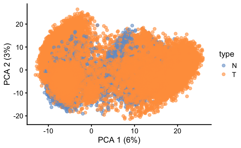

This is quite an abrupt cut-off, but I’m already running far too long and my creativity is also long gone. If you want to know more, like, comment, and subscr - no, that’s the wrong platform.

To be continued… maybe, if I’m bored enough.

And you’ve finally made it through, thank heavens.

Congratulations! You’re probably feeling pretty dang hydrated, if you followed my instructions at the beginning. I know the topic isn’t one a lot of you data science people will be using in the future, but I hope it was at least more interesting than watching paint dry on a snail.

To summarize: in this exceedingly long post, I forcibly took you on a whirlwind tour through Single-Cell Experiment (SCE) objects in R, exploring their structure, how they store complex biological data, and ways to wrangle that data into something manageable. We covered normalization techniques to make the data usable, identified highly variable genes to focus our analysis, and briefly dunked our toes into Principal Component Analysis (PCA) to visualize it all. Hopefully, this introduction gave you a basic understanding of SCE objects and how they can be used to make sense of cellular gene expression data.

If you are morbidly curious about SCEs and their applications, this link will take you to a much better guide to scRNA-seq data analysis. If you have any questions, feel free to ask, though I unfortunately am young and inexperienced and thus have many gaps in my knowledge.

Now, you have my permission to depart and never return to this post. Ciao!

Links…

…to avoid being copyrighted, sent to prison for ten years, and then returning to find my college education is obsolete and I have $200,000 in student loans to pay back but then instead of doing that I just jump off a bridge but then I survive and have to pay the medical bills as well and so I end up homeless and penniless under that same bridge in a cruel twist of fate and resort to talking about SCE objects as my busking method which somehow leads to me giving any money I have to the poor souls who walk by me and then I perish

Figure 1 Figure 2